Category: Quantum Computing

A quantum circuit drawn on a screen can connect any two abstract qubits with a line. A processor cannot necessarily do the same. Real devices support particular operations on particular physical qubits, often only between certain neighboring pairs. Before an algorithm runs, software has to rewrite its neat diagram into instructions the chosen machine can execute.

That rewrite is usually called compilation or transpilation. It may add operations, move the circuit onto a different set of qubits, and change its timing. The result can determine whether an experiment is feasible on noisy hardware, even though the processor’s advertised qubit count has not changed.

One circuit, two kinds of qubits

The qubits in an abstract circuit are virtual placeholders for its work. Today’s hardware exposes physical qubits with locations, connections and device-specific behavior. A compiler first chooses which physical qubit will represent each circuit qubit. In Qiskit this is the layout stage, described in IBM Quantum’s current transpilation guide.

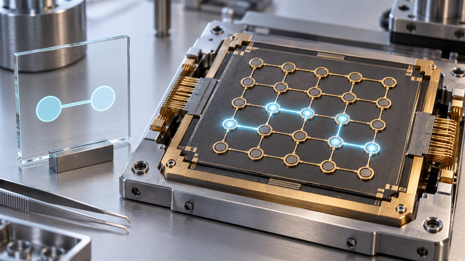
Imagine a circuit whose first and last qubits must interact. If the corresponding physical qubits are far apart on a chip that permits only neighboring two-qubit gates, that requested interaction cannot be issued as drawn. Choosing a better initial placement might bring them together. Otherwise the compiler must route quantum information through allowed connections, commonly by adding SWAP operations or an equivalent rewriting.

This is one reason a larger processor does not automatically give every circuit a better home. Its useful connections and the quality of the available physical qubits matter too. Our earlier article on quantum benchmarks beyond qubit count discusses the broader comparison problem.

The chip’s connection map sets the route

A coupling map is a graph of physical qubits and permitted two-qubit interactions. IBM’s hardware-representation guide shows how a poor layout can require extra SWAPs while a layout that matches the circuit’s structure can avoid them in the illustrated example. Those extra gates are not merely a cosmetic difference on noisy hardware: they add opportunities for error and can lengthen the circuit.

Connectivity is not identical across platforms. Google’s Cirq hardware documentation describes a grid on which two-qubit operations are restricted to adjacent sites. That does not mean every quantum processor has the same grid, or that every possible interaction is available at equal quality. A compilation claim is meaningful only in the context of a particular target device and its supported operations.

Routing itself is an optimization problem. The compiler can search for a path with fewer additional operations, but it may also have to consider which physical links are less noisy. Two compilations of the same abstract circuit can therefore produce different physical circuits without changing the intended computation.

Abstract gates must become native instructions

A circuit library may let a developer express a convenient gate that the processor does not implement directly. Translation decomposes it into the device’s supported basis gates. IBM’s documentation gives examples of a target instruction set that includes specific single-qubit operations, an entangling gate, measurements and resets. The compiler must also respect the target’s connectivity and any supported control-flow rules.

Google’s Cirq documentation likewise notes that unsupported gates need an equivalent decomposition into the device’s available set. A circuit that looks shorter before translation can grow after it is expressed in hardware instructions. Counting high-level gates without showing the compiled result can therefore hide a substantial part of the workload.

Some operations are effectively bookkeeping rather than a physical pulse on particular machines. Google’s documentation describes virtual Z rotations that are tracked in the compiler and generally add no direct gate duration. That detail is device-specific; it is a reminder that two circuits with the same number of symbolic gates need not take the same time.

Scheduling matters after mapping

Once operations are legal, they still need an execution order. Independent gates may run at the same time; gates on the same qubit cannot be scheduled as though they were independent. Idle intervals can matter because a qubit does not wait perfectly while other work proceeds. Qiskit’s staged transpiler includes an optional hardware-aware scheduling stage for making circuit timing explicit.

Optimization can cancel redundant operations, select a different decomposition or search for a better placement. But a higher optimization setting is not a free upgrade. IBM notes that stronger preset optimization generally takes longer to compile, and its SABRE tutorial shows that a specialized rewrite can beat a general-purpose routing heuristic for a circuit with known structure.

Compiler performance therefore has at least two costs: the classical time spent finding a physical circuit and the quantum resources used when that circuit runs. A heavily optimized circuit may be worth the compilation time if reused many times; a one-off experiment may present a different tradeoff. That is an inference from the workflow, not a benchmark result from our own testing.

How to compare compiled circuits honestly

Useful comparisons start with the same algorithmic task and name the target processor. They report physical qubits used, two-qubit gate count, circuit depth, and ideally timing or an error-aware performance measure. They also state whether a result came from real hardware, a noiseless simulator or a simulator using a hardware noise model.

There is no single magic number. Fewer gates may reduce one source of error but place work on a worse physical link. Lower depth may help one processor while increasing another operation that matters more. Device calibration and supported gate sets can change the best route. Google’s device guide explicitly cautions that gate behavior varies by qubit and can drift over time.

For a larger algorithm, the compiled circuit is just one piece of a full quantum resource budget. An attractive diagram that leaves out routing and native-gate translation is not yet a hardware execution plan.

Limits of compilation and what to watch next

A compiler cannot manufacture a missing reliable interaction or turn a noisy device into an error-corrected one. It can choose among available implementations and sometimes make much better use of them. Even then, observed output still needs careful interpretation; error mitigation is a separate layer with different limits.

Watch for clearer reporting of the circuit after compilation, not just its abstract form. Better device models, calibration-aware mapping and specialized rewrites could make more algorithms practical, but claims should be compared on equivalent workloads and measured outcomes. For readers evaluating a quantum demonstration, the useful question is simple: what did the hardware actually execute? This article explains published documentation and does not claim hands-on access to a quantum processor.

Primary and authoritative sources

• IBM Quantum: Introduction to transpilation
• IBM Quantum: Represent quantum computers for the transpiler
• IBM Quantum: Transpilation optimization with SABRE
• Google Quantum AI: Google devices in Cirq

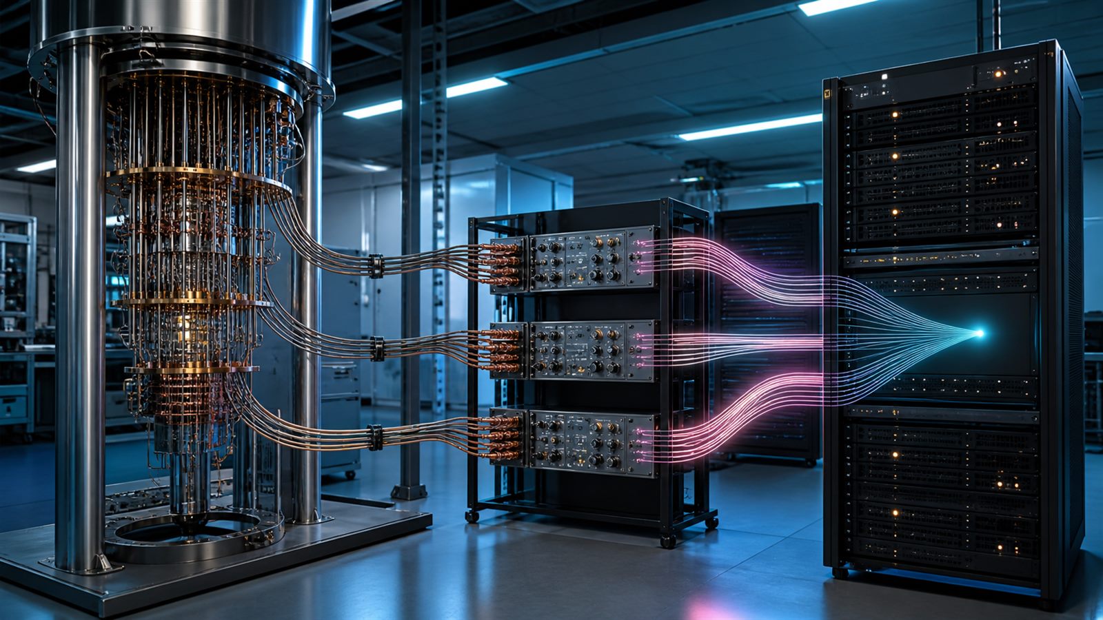
Featured image is an AI-generated editorial metaphor, not a photograph of a named quantum processor.

Quantum sensors are often introduced with one irresistible promise: they can detect signals that conventional instruments miss. That is true in important cases, but it is not a universal upgrade. A sensor that excels at the faintest magnetic field may require shielding or cooling. Another may survive harsh conditions but give up some sensitivity. A third may measure acceleration with exquisite stability while demanding lasers, vacuum hardware, and careful vibration control.

The practical question is therefore not whether a sensor is quantum. It is whether its complete measurement system delivers the right sensitivity, range, speed, resolution, stability, and reliability for a particular job. Quantum physics can improve one or more of those metrics, but engineering determines whether the advantage survives outside the laboratory.

A quantum sensor is a measurement architecture

A quantum sensor uses a controlled quantum property of matter or light to infer a physical quantity. According to NIST’s quantum sensing overview, examples include atomic clocks, magnetometers based on atomic spin or superconductivity, single-photon detectors, atom interferometers, electric-field sensors, and squeezed-light instruments.

The sensing element is only the center of the architecture. Lasers prepare and read atomic states. Microwave sources manipulate spins. Photodetectors convert light into electrical signals. Control software estimates a quantity from noisy data. Enclosures manage temperature, vibration, stray fields, and contamination. Packaging, power, and communications decide whether the instrument can leave a specialist laboratory.

This is similar to the broader shift described in quantum hardware manufacturing: performance depends on repeatable subsystems and interfaces, not only on an impressive device demonstrated once.

Sensitivity is only one line on the specification sheet

Sensitivity describes how small a change can be detected under stated conditions, usually over a defined bandwidth and integration time. It is not the same as accuracy, which concerns closeness to the true value. Nor is it resolution, repeatability, long-term stability, spatial resolution, or immunity to interference.

A very sensitive instrument can still be unsuitable if its useful range is narrow, its response is slow, or its reading drifts when temperature changes. Longer averaging can reveal weaker signals, but that may hide fast events. Increasing interaction time can improve precision, yet also make the quantum state more vulnerable to environmental noise. Every published sensitivity number needs context: frequency, measurement time, operating temperature, geometry, and the noise conditions under which it was obtained.

Magnetometers make the tradeoffs visible

NIST’s comparison of quantum magnetometers shows why no single platform wins every application. Superconducting quantum interference devices, or SQUIDs, are exceptionally sensitive and support uses from brain imaging to materials research. Their superconducting circuits, however, require cryogenic refrigeration, which adds cost, mass, and operational complexity.

Atomic vapor magnetometers use laser light to prepare and read the spins of atoms in a glass cell. They can approach SQUID-class sensitivity while operating near room temperature, which makes portable biomedical and geophysical instruments more plausible. But they still need stable optical control and protection from unwanted magnetic fields.

Diamond nitrogen-vacancy, or NV-center, sensors offer another balance. The sensing defects are embedded in durable diamond, can work over broad temperature and pressure conditions, and can provide nanoscale magnetic images. NIST notes that the best NV magnetometers have not matched the weakest-field sensitivity of leading atomic and SQUID systems, but they handle high-frequency fields and a wide range of field strengths well. That can be the better capability for chip inspection, microscopy, or rugged navigation experiments.

Bandwidth and dynamic range decide what can be observed

A sensor must respond on the time scale of the phenomenon. A device optimized to average a nearly constant field for minutes is different from one designed to capture radio-frequency changes. Likewise, dynamic range determines whether the instrument can distinguish a tiny variation without saturating when the background is large.

A 2025 NIST review of atom-based electromagnetic sensing covers vapor-cell, NV-center, and Rydberg-atom modalities spanning direct-current fields through terahertz frequencies and spatial scales from nanometers to meters. That range is evidence of specialization, not interchangeability. Buyers should compare performance in the frequency band, geometry, and field strength that their application actually uses.

The environment becomes part of the instrument

Quantum states are useful because they respond to small disturbances. The same fact makes them respond to disturbances that are not the target signal. Stray magnetic fields, laser-frequency noise, vibration, temperature gradients, and mechanical motion can all appear in the output unless the instrument suppresses or models them.

Atom interferometers illustrate the point. They split and recombine matter waves so that gravity, acceleration, or rotation changes the interference pattern. NIST describes potential applications in gravimetry and navigation, but the apparatus relies on cooled atoms, controlled laser pulses, and a stable measurement reference. The sensor does not remove vibration and platform motion from the world; the system must separate those effects from the quantity being measured.

An atomic reference does not validate the whole device

Atoms of the same isotope have reproducible energy levels, giving many quantum sensors an intrinsic and highly consistent reference. That is one reason optical clocks can support a future redefinition of the second.

However, a complete field instrument also contains optics, electronics, geometry, algorithms, and environmental compensation. Those components can introduce offsets and uncertainty. Traceability therefore requires an uncertainty budget and comparisons against trusted standards, not simply a statement that the sensing element is atomic. Self-referencing can reduce calibration burden without making validation unnecessary.

Field deployment is an engineering program

The U.S. National Quantum Initiative’s strategy for bringing quantum sensors to fruition emphasizes testing prototypes with end users and developing enabling components such as compact, reliable lasers and integrated optics. Those recommendations recognize that laboratory sensitivity is only one step toward a deployable product.

A field system must start reliably, survive transport, maintain alignment, reject interference, report its health, and recover from ordinary faults. It also needs a useful size, weight, power draw, maintenance interval, and cost. In many applications the best design will combine a quantum sensor with classical inertial sensors, magnetic sensors, timing references, or statistical filters. The classical system supplies continuity and range; the quantum channel supplies a precise correction or reference.

How to evaluate a quantum sensing claim

Begin with the quantity being measured and the decision the measurement supports. Then ask for sensitivity and accuracy over the required bandwidth, dynamic range, spatial resolution, warm-up time, and long-term drift. Check whether the quoted result was obtained in shielding, vacuum, or cryogenic conditions and whether those conditions exist in the intended deployment.

Look for comparisons against the best relevant classical instrument, not against an outdated baseline. Ask whether the result covers the sensing element alone or the complete packaged system. Independent repeatability, uncertainty analysis, and field trials matter more than the word quantum on a product page. The same discipline applies to quantum random-number generators, where certification must evaluate the whole source and its failure behavior.

Limitations and what to watch next

Quantum sensors will not replace inexpensive classical sensors where existing performance is already sufficient. Some platforms remain research instruments, and even mature quantum devices can depend on costly support equipment. Security-sensitive navigation claims also require testing against spoofing, magnetic anomalies, map errors, and deliberate interference; a sensitive detector alone does not create a trustworthy navigation service.

Watch for integrated photonics, smaller laser and vacuum packages, better magnetic shielding, robust calibration procedures, and published field comparisons using common metrics. The most important progress may look less dramatic than a record sensitivity number: a sensor that operates for months, reports honest uncertainty, and solves one measurement problem better than the complete classical alternative.

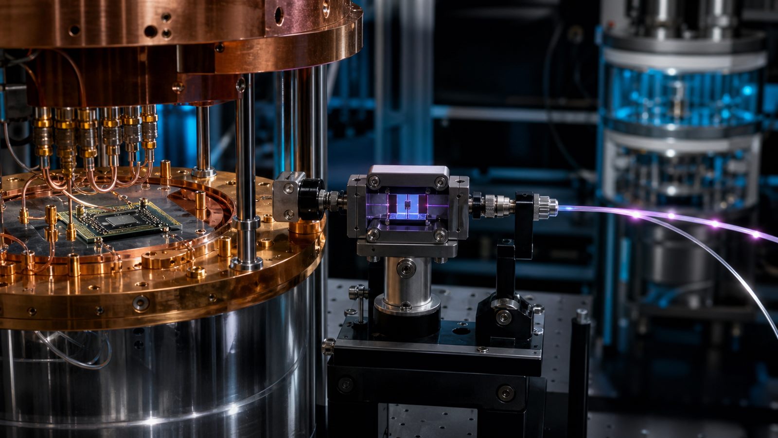
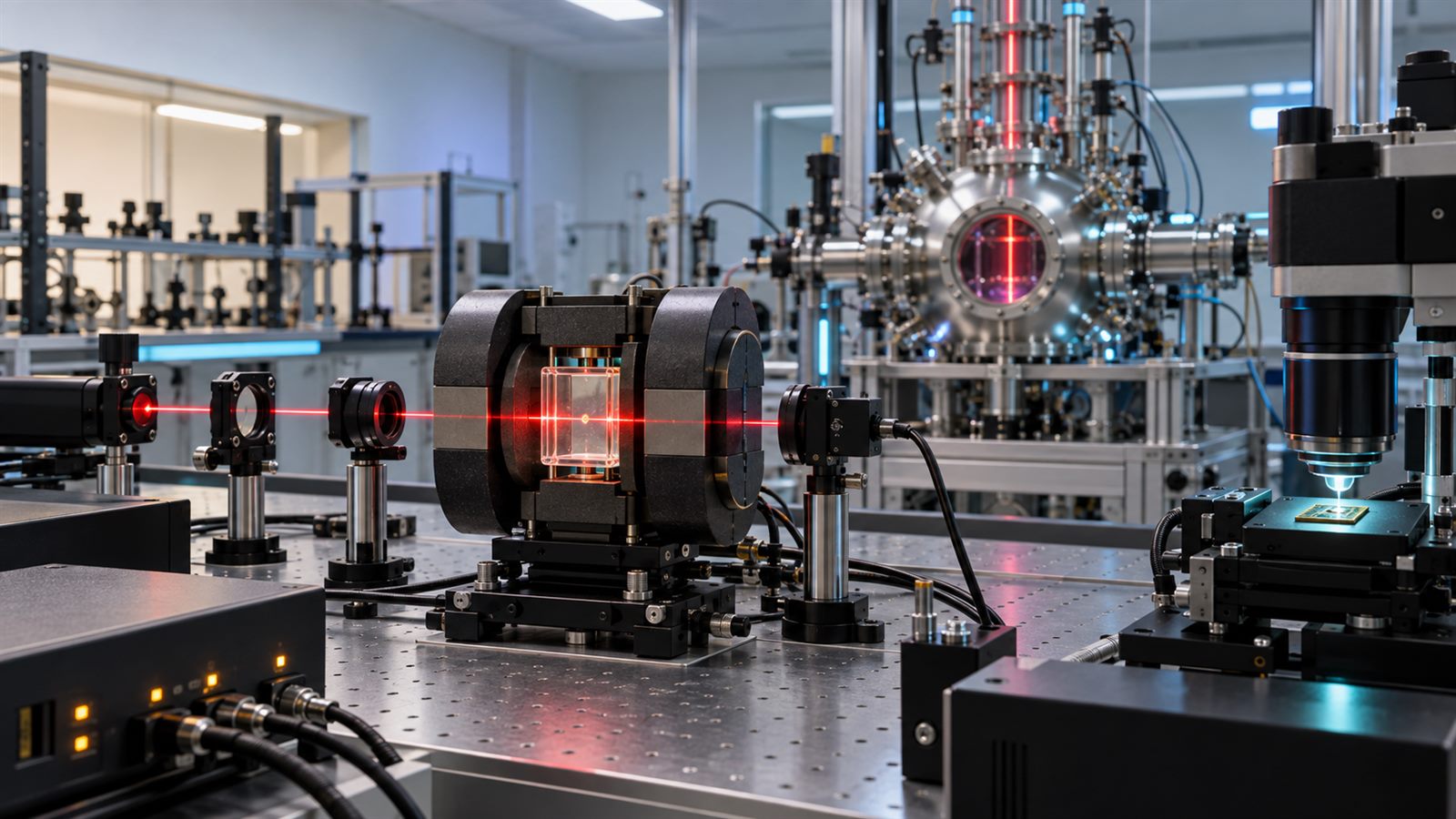
Featured image: AI-generated editorial visualization of several quantum sensing platforms in a precision laboratory. It is not a photograph of a specific experiment or a hands-on product test.

Primary and authoritative sources

• NIST: Quantum Sensing Explained
• NIST: Sensors for a Magnetic World
• NIST: Atom-Based Quantum Sensing of Electromagnetic Fields
• NIST: Turning Atoms Into Waves to Measure Gravity and Acceleration
• National Science and Technology Council: Bringing Quantum Sensors to Fruition

Quantum annealers and gate-model quantum computers are often discussed as though they were competing versions of the same machine. They are not. Both use quantum physics, but they expose very different ways to describe a problem, control hardware, and judge a useful result. That distinction matters whenever a headline compares qubit counts or claims that one architecture has solved an optimization problem faster than another.

A quantum annealer is a specialized system for exploring low-energy configurations of a mathematical model. A gate-model machine applies a programmed sequence of quantum operations, or gates, to qubits before measuring them. One is closer to a configurable physical optimizer; the other is closer to a programmable quantum processor. Neither description automatically makes one superior. It means that comparisons must include the problem formulation, hardware restrictions, classical support work, solution quality, and total elapsed time.

Quantum annealing begins with an energy landscape

Many optimization tasks can be written as a quadratic unconstrained binary optimization problem, usually shortened to QUBO, or as an equivalent Ising model. The variables take binary values, while linear and pairwise terms assign a score to every possible configuration. Lower scores correspond to lower energy. The job is to find the minimum, or at least a sufficiently low-energy answer.

In a superconducting quantum annealer, programmable biases influence individual qubits and couplers define relationships between connected qubits. The system begins under an initial Hamiltonian, a mathematical description of its energy, and gradually shifts toward the problem Hamiltonian. According to D-Wave’s technical introduction to quantum annealing, the measured bit string at the end represents a low-energy state of the submitted problem. Repeating the process produces a collection of candidate solutions rather than a guaranteed perfect answer in every run.

This architecture can also be used for sampling low-energy states, where the goal is not necessarily one optimum. That makes annealing relevant to some probabilistic and physics problems as well as scheduling, routing, allocation, and other combinatorial tasks.

Gate-model computers execute circuits

A gate-model computer takes a different route. A developer expresses an algorithm as a circuit containing single-qubit and multi-qubit operations. A compiler then maps those operations onto the gates and connections supported by a specific processor. Measurement converts the final quantum state into classical results, and many circuit repetitions are normally required to estimate probabilities.

This circuit abstraction can represent a much broader range of algorithms, including quantum simulation, phase estimation, search routines, and error-corrected programs. It also brings familiar engineering constraints. Google’s Cirq documentation shows that circuits must be transformed for a device’s available operations and connectivity. On current hardware, noise and limited circuit depth restrict how much useful computation can be completed before errors dominate.

The long-term gate-model goal is a fault-tolerant computer built from logical qubits. That is why raw physical-qubit comparisons can mislead, as our guide to full quantum resource estimates explains. An annealer with many specialized qubits and a gate-model processor with fewer programmable qubits are not interchangeable capacity figures.

Problem mapping can consume the apparent scale

A real optimization problem rarely matches an annealer’s hardware graph perfectly. If two logical variables must interact but their physical qubits are not directly connected, the mapping process may represent one logical variable with a chain of physical qubits. This is called minor embedding. Longer chains consume hardware, introduce additional parameters, and can break into inconsistent values that require interpretation.

Gate-model processors have a related mapping cost. A compiler may add swap operations to bring nonadjacent qubits together, increasing circuit depth and exposure to noise. The details differ, but both architectures demonstrate the same lesson: the number of hardware qubits does not equal the size of a useful application. Topology, control precision, and mapping overhead determine how much of the machine a problem can actually use.

The fastest quantum step is not the full runtime

Quantum anneals can be extremely short, but quoting only the annealing interval leaves out important work. The system must be programmed, allowed to settle, annealed, read out, and often sampled repeatedly. D-Wave’s operation and timing documentation separates programming time, per-sample anneal time, readout time, delay, and total QPU access time.

An application also pays for classical steps outside the processor: converting business constraints into a QUBO, embedding the model, choosing penalty weights, decoding chains, evaluating candidate answers, and possibly iterating through a hybrid solver. Gate-model workflows similarly include circuit compilation, queueing, repeated shots, error processing, and classical optimization. A fair performance claim must state which of those stages are included.

Optimization results need more than one stopwatch

Optimization is usually about the trade-off between time and answer quality. Two solvers may reach different objective values, or one may find a good answer quickly while another improves for longer. A useful benchmark therefore reports the best-known value, the gap from that reference, the distribution across repeated runs, problem size, and time to reach a defined target.

A peer-reviewed Los Alamos National Laboratory study compared quantum annealing and gate-model approaches on Max-Cut problems by tracking solution quality as a function of time. Its framework is valuable because it treats performance as a profile, not a single winner-takes-all number. The same discipline is central to our earlier discussion of independent quantum benchmarks.

Classical baselines must be strong and problem-specific

A quantum result has little meaning without a capable classical comparison. Generic simulated annealing may be a useful reference, but it is not always the best classical method for a structured scheduling, graph, or constraint problem. Modern mixed-integer solvers, graph algorithms, tensor-network methods, GPU heuristics, and carefully tuned domain-specific techniques can set much tougher baselines.

The comparison must also use equivalent objectives and constraints. A simplified QUBO may be easier to run on quantum hardware but may omit details that a production classical model handles. Data loading and solution validation belong in the accounting. Researchers should publish enough information to reproduce the instances, parameter choices, hardware access assumptions, and stopping rules.

Where quantum annealing fits today

Annealers are useful research platforms for testing optimization formulations, sampling energy landscapes, studying quantum dynamics, and building hybrid workflows. NASA’s Quantum Artificial Intelligence Laboratory investigates optimization and hybrid quantum-classical algorithms for areas such as planning, scheduling, flight-gate assignment, and trajectory deconfliction. NASA also emphasizes physics-inspired classical methods that can work at application scale now.

That is a more realistic picture than either extreme of the public debate. Quantum annealing is not a universal replacement for classical optimization, but it is also not simply a failed version of a gate-model computer. It is a specialized architecture whose value depends on whether a problem maps well to its energy function and connectivity, and whether the complete system improves a meaningful metric.

Important limitations and common misconceptions

An annealer does not automatically find the global optimum. Thermal effects, control errors, small energy gaps, embedding choices, and finite sampling can move results away from the ground state. More physical qubits do not erase those constraints. Likewise, a gate-model machine’s greater programmability does not mean current noisy hardware can run every theoretically known algorithm at a useful scale.

It is also unsafe to assume that an optimization problem is a good quantum candidate merely because it is difficult. Structure matters. Some hard-looking instances yield quickly to specialized classical techniques, while a compact mathematical model may become much larger after hardware mapping. Claims of advantage should survive strong baselines, repeated tests, and independent access to the same workload.

What to watch next

The most informative progress will come from denser and more controllable hardware graphs, lower analog error, better embedding tools, and benchmark reports that publish end-to-end timing and solution distributions. Cross-model studies should compare annealers, gate-model algorithms, and leading classical solvers under the same target-quality rules.

For readers, the practical filter is simple: ask what mathematical problem was submitted, how much mapping was required, which runtime stages were counted, how answer quality was measured, and which classical methods were challenged. Those questions reveal far more than the qubit total. Quantum annealing and gate-model computing can both advance, but they should be judged as distinct tools rather than different-sized versions of one machine.

Primary and authoritative sources

• D-Wave: What Is Quantum Annealing?
• D-Wave: Operation and Timing
• Google Quantum AI: Introduction to Cirq
• Los Alamos National Laboratory: Optimization Applications as Quantum Performance Benchmarks
• NASA Quantum Artificial Intelligence Laboratory

The second is currently defined by exactly 9,192,631,770 periods of microwave radiation associated with a transition in cesium-133 atoms. That definition has supported global timekeeping, satellite navigation, telecommunications, and precision science since 1967. It is not suddenly inaccurate.

Optical atomic clocks can nevertheless divide time more finely. Their atoms respond to light oscillating hundreds of trillions of times per second, giving physicists a much faster reference than a microwave transition. The best optical clocks now outperform cesium standards, but a world definition cannot be chosen from a single laboratory record. It needs independent clocks, dependable comparisons, gravity corrections, sustained operation, and international agreement.

Optical frequency provides a finer ruler

An atomic clock does not count a mechanical pendulum. A controlled electromagnetic signal probes an atomic transition, and feedback keeps an oscillator aligned with that transition. The current cesium definition uses a microwave transition; an optical clock uses a much higher-frequency transition in an atom or ion.

More oscillations per second create a finer scale on which to locate the center of a transition. According to the NIST overview of optical clocks, this higher frequency is a central reason optical systems can achieve better stability and accuracy. A frequency comb bridges the gap between optical light and electronic counters by linking a laser’s frequency to a measurable series of evenly spaced lines.

Accuracy and stability are related but different. Accuracy describes how closely a clock realizes its unperturbed atomic frequency after systematic shifts are evaluated. Stability describes how quickly repeated measurements settle toward a consistent value. A clock can be exceptionally stable over short periods while still carrying a systematic bias.

Lattice clocks and ion clocks make different tradeoffs

Optical lattice clocks trap thousands of neutral atoms in a standing wave of laser light. Measuring many atoms produces a strong signal and can improve short-term stability, but the lattice, atom density, temperature, magnetic fields, and probe light must be controlled.

Single-ion clocks isolate one charged atom in an electromagnetic trap. The ion can be shielded from many interactions, supporting very low systematic uncertainty, while its single-particle signal can require longer averaging. Candidate species include strontium and ytterbium in lattice clocks and aluminum or ytterbium ions in ion clocks.

These systems are quantum sensors already operating beyond the laboratory concept stage. Our broader guide to quantum sensors before fault-tolerant quantum computers explains why precision measurement is one of quantum technology’s most mature applications.

A record clock is not automatically a definition

A national measurement system must be reproducible in more than one facility. Researchers need to build independent clocks based on the same transition, evaluate systematic effects using different equipment, and obtain consistent frequencies. They also compare ratios between different optical transitions. Ratios reveal disagreements without requiring either clock to be treated as the final definition.

A 2026 NIST report on optical frequency ratios compared aluminum-ion, ytterbium, and strontium clocks with uncertainties at or below 3.2 parts in 10¹⁸. The clocks were connected across a 3.6-kilometer phase-stabilized fiber link. The authors also noted discrepancies with some previous measurements, which is exactly why repeated, independent comparisons are essential.

A definition should not depend on one instrument’s undocumented correction or one laboratory’s local environment. Agreement across species and institutions tests both the clocks and the measurement methods used to evaluate them.

Time transfer must preserve the clocks’ performance

Two superb clocks cannot be compared through a link that adds more noise than the difference being measured. Optical fiber can transfer stable light between laboratories, using active compensation to suppress phase changes caused by temperature and vibration. Fiber networks are powerful but geographically limited and require carefully monitored equipment.

Satellite links can connect distant regions, yet traditional microwave time transfer generally lacks the precision needed to expose the smallest optical-clock differences quickly. Optical satellite links and transportable clocks are active development areas. The networking challenge has parallels with quantum networks and repeaters, although optical-clock comparison does not require an entanglement-based quantum internet.

Comparison infrastructure must also report interruptions and uncertainty. A spectacular short measurement is not equivalent to a link that supports routine international timekeeping.

Gravity changes the rate of a clock

General relativity predicts that a clock at higher gravitational potential runs faster than one lower down. At optical-clock precision, elevation and the local distribution of mass can no longer be treated as minor details. Comparing clocks in different buildings or countries requires knowledge of their gravitational potential, not simply their height above an approximate sea level.

This sensitivity can become a measurement tool called chronometric geodesy. Networks of optical clocks may help detect differences in gravitational potential and improve height systems. But the same physics is first a correction problem: laboratories need geodetic surveys and models accurate enough that gravity does not masquerade as a clock error.

UTC needs reliable clocks, not occasional demonstrations

Coordinated Universal Time, or UTC, is calculated from an international ensemble of atomic clocks. A future optical definition must connect to that operational system. Optical clocks therefore need better uptime, automated recovery, documented maintenance, and regular frequency reports, not just low uncertainty during a carefully selected experiment.

The international roadmap toward redefining the second identifies contributions to UTC, clock comparisons, gravitational-potential knowledge, and mandatory performance criteria among the open tasks. These requirements make the project an infrastructure transition as much as a physics decision.

The world must choose what the new definition names

One option is to select a single optical transition in one atomic species. That would be conceptually similar to the present cesium definition and give laboratories a clear target. It could also concentrate dependence on the practical challenges of one clock architecture.

Another option is to define the second using an ensemble or weighted combination of multiple optical transitions. That could draw strength from several mature clock types, but it would create a more complex definition and require maintained frequency ratios between species. The BIPM redefinition FAQ presents both approaches as options under consideration.

The decision also needs continuity. The length of the second should not jump when the wording changes. Existing cesium clocks, time scales, and calibrated equipment must remain traceable through the transition.

Consumers should expect continuity, not a visible clock change

A redefinition would improve the foundation of measurement, not make a phone display seconds differently. National laboratories would realize the new definition and connect it to UTC; networks, navigation systems, exchanges, and devices would continue distributing time through existing layers.

Benefits would appear first where tiny frequency errors matter: fundamental physics, geodesy, navigation research, radio astronomy, and calibration. Broader systems may eventually gain more resilient synchronization and better positioning, but those outcomes require distribution infrastructure as well as better laboratory clocks.

Claims should be evaluated with the same discipline used for other quantum devices. Independent replication, uncertainty budgets, uptime, and traceability matter more than a single impressive digit. Our article on quantum random-number certification explains why a quantum label does not remove the need to test the complete system.

What to watch next

The BIPM roadmap says the international metrology community is working toward a possible redefinition around 2030. Before then, watch for more independent optical frequency ratios, long-distance comparisons, routine contributions from optical clocks to UTC, improved gravitational-potential measurements, and agreement on mandatory criteria.

The decisive milestone will not be another record in one laboratory. It will be a network of clocks that different countries can build, compare, operate, and trust while preserving continuity with the timekeeping system the world already uses.

Primary and authoritative sources

• BIPM: Roadmap for the Redefinition of the Second
• BIPM: Frequently Asked Questions on Redefining the Second
• NIST: Optical Clocks, the Future of Time
• NIST: Roadmap Towards the Redefinition of the Second
• NIST: Optical Clock Frequency Ratios at 3.2 Parts in 10¹⁸

Quantum processors are noisy: gates are imperfect, qubits lose coherence, measurements make mistakes, and calibration drifts. Full quantum error correction aims to protect logical information by detecting and correcting faults during a calculation. Quantum error mitigation takes a different route. It runs noisy circuits, often many times and in several modified forms, then uses classical analysis to estimate what a less noisy result would have been.

That can improve selected measurements on today’s hardware without encoding every logical qubit across a large error-correcting system. It does not repair the quantum state inside the processor, extend a circuit indefinitely, or guarantee a correct answer. Understanding that boundary is essential when a demonstration claims useful computation before fault tolerance.

Mitigation improves an estimate after the experiment

A quantum algorithm usually ends with repeated measurements. Each run produces a bit string, while many runs provide statistics. Researchers often want an expectation value: the average value of a measurable quantity such as energy, magnetization, or another observable. Error mitigation changes how those statistics are collected or interpreted.

The distinction from correction is physical. Error correction encodes information across multiple qubits, repeatedly measures error syndromes, and applies or tracks corrections while preserving the logical state. Mitigation normally leaves the noisy physical computation in place. It estimates a cleaner output from additional executions, noise knowledge, symmetries, or classically tractable reference circuits.

The broad Review of Modern Physics survey of quantum error mitigation describes a family of methods rather than one universal filter. Each method has assumptions about the noise, target quantity, circuit, and classical resources. Those assumptions determine whether an improved number is credible.

Readout mitigation addresses measurement mistakes

A processor may prepare the right final state but report some zeros as ones or ones as zeros. A calibration experiment can estimate a response matrix for the measurement system. Software then uses that model to infer a distribution closer to the one that existed before readout error.

This is useful, but the calibration matrix grows with the system if correlations between qubits matter. A simplified model may treat readout errors as independent when they are not. The device can also drift between calibration and the real experiment. Readout mitigation corrects only the final measurement channel; it does not undo errors accumulated during the circuit.

Symmetry checks can reject impossible outcomes

Some problems have known constraints. A physical model may conserve particle number, parity, or another symmetry. If a measured outcome violates that rule, the experiment can discard it or use the violation rate as evidence of noise. This technique can improve results without a complete hardware noise model.

Postselection has a cost because rejected shots carry no final estimate. It can also hide problems if the analysis reports only retained data without showing the acceptance rate. Symmetry verification catches errors that leave the allowed subspace, but errors within that subspace can remain invisible.

Zero-noise extrapolation deliberately makes noise stronger

Zero-noise extrapolation, or ZNE, runs related versions of a circuit at several effective noise strengths. If researchers can amplify noise in a controlled way without changing the ideal computation, they can fit the measured values and extrapolate back toward a hypothetical zero-noise point.

IBM’s technical tutorial demonstrates this workflow using probabilistic error amplification. Other approaches can stretch control pulses or fold extra gate pairs into a circuit. The method does not create a truly noiseless run; it estimates an intercept from noisy points.

The quality of that estimate depends on the chosen noise factors, fitting model, number of shots, and whether amplification preserves the relevant noise structure. Extrapolation can magnify statistical fluctuations. If the device drifts or different error mechanisms scale differently, a smooth fit may look convincing while remaining biased.

Probabilistic cancellation trades noise for sampling cost

Probabilistic error cancellation characterizes noisy operations and represents an ideal operation as a weighted combination of operations the hardware can perform. The processor samples from those implementable circuits, and classical post-processing combines their results with positive and negative weights.

Under an accurate noise model, the resulting expectation-value estimator can be unbiased. The difficulty is variance. Cancellation weights can make the estimator noisy, requiring many more circuit executions to reach a useful confidence interval. As circuits grow deeper or noisier, that sampling overhead can become prohibitive.

A 2023 Nature Physics experiment on scalable mitigation reported competitive expectation values on larger noisy circuits and analyzed the associated overhead. It is evidence that mitigation can work in carefully characterized regimes, not proof that any large circuit can be cleaned cheaply.

More circuit executions are the hidden resource

Error correction is famous for needing many physical qubits per logical qubit. Mitigation avoids much of that spatial overhead but consumes other resources: circuit shots, calibration experiments, device access time, classical processing, and uncertainty analysis. A mitigated result should therefore include the total number of executions and not only the final error bar.

Noise can erase information that post-processing cannot recover efficiently. A 2024 Nature Physics analysis of mitigation limits showed strong worst-case sampling barriers for broad classes of methods. The result does not say every practical circuit is hopeless. It says there is no general promise that mitigation will scale efficiently as systems and circuit depth increase.

This is why a full quantum resource estimate should identify shots, calibration, classical reconstruction, and validation alongside qubits and gates. A short circuit with a favorable observable may be practical even when a deeper general computation is not.

Evidence of utility still needs a trusted reference

In 2023, researchers reported evidence for utility before fault tolerance using a noisy 127-qubit processor and error mitigation. They checked the method with exactly verifiable circuit instances and compared results with leading classical approximations. The study helped define a serious experimental path, while also illustrating how much validation is required.

A quantum result is not established simply because one classical method struggles. Researchers need multiple classical baselines, instances with known answers, withheld tests, uncertainty intervals, sensitivity to analysis choices, and enough information for independent reproduction. Classical algorithms also improve, so a claimed boundary can move after publication.

Our guide to independent quantum benchmarks explains why vendor-controlled tests are insufficient. Error mitigation adds another layer that evaluators must audit: the raw noisy data, noise model, discarded shots, amplification schedule, estimator, and total computational cost.

Mitigation and correction can work together

The choice is not permanently either mitigation or correction. Error suppression can improve hardware and control before a circuit runs. Small error-detecting or error-correcting codes can protect part of a computation. Mitigation can then reduce residual bias in logical measurements. The most useful stack may combine all three at different layers.

Only error correction offers a path to arbitrarily long reliable computation when physical error rates, code behavior, decoding, and system operation satisfy the required conditions. Our article on quantum error correction as an engineering benchmark focuses on that scaling test. Mitigation is valuable precisely because the field has not yet completed it.

What readers should demand from a mitigated result

A credible report should identify the observable being estimated, baseline hardware error, mitigation method, assumptions, calibration timing, number of raw and retained shots, uncertainty interval, and unmitigated result. It should show performance across more than a single favorable instance and explain how answers were verified.

Readers should be cautious when a paper reports improvement without total execution cost, uses the same circuits to tune and validate the estimator, omits failed instances, or compares against a weak classical baseline. A smaller error bar does not rule out systematic bias from an inaccurate noise model.

What to watch next

Progress will come from lower-noise hardware, faster execution, better drift tracking, compact noise models, transparent uncertainty accounting, and benchmarks that compare mitigation methods under the same conditions. Logical-qubit experiments will also test whether mitigation remains useful after partial error correction.

Quantum error mitigation is best understood as scientific inference under difficult noise, not a software repair button. It can extract a better estimate from a limited experiment, sometimes impressively. The result earns trust only when the extra sampling, assumptions, verification, and remaining uncertainty are visible.

Primary and authoritative sources

• Review of Modern Physics: Quantum Error Mitigation
• Nature Physics: Scalable Error Mitigation for Noisy Quantum Circuits
• Nature: Evidence for Utility Before Fault Tolerance
• Nature Physics: Limitations of Quantum Error Mitigation
• IBM Quantum Documentation: Probabilistic Error Amplification

Superconducting quantum processors speak in microwaves. Optical fiber carries information most effectively as light. Connecting those two worlds is not a matter of plugging in a different cable: a quantum transducer must convert a fragile state without measuring it, copying it, or burying it in noise.

That requirement makes microwave-to-optical transduction one of the most consequential hardware problems in modular quantum computing. A useful device could let separate cryogenic processors share quantum states over fiber, reducing the need to force every qubit into one refrigerator. It could also provide an interface between processors and the longer-distance links described in our guide to quantum networks and repeaters. Laboratory progress is real, but a transducer that works in one carefully tuned experiment is still far from a dependable network component.

Why microwave qubits and optical fiber do not naturally match

Many leading superconducting circuits store and manipulate quantum information at microwave frequencies, typically inside a dilution refrigerator at temperatures close to absolute zero. Microwave control fits the electrical nature of those circuits, but microwave photons are awkward travelers. At ordinary temperatures, thermal background energy can overwhelm single microwave photons. Coaxial cables also conduct heat into a refrigerator, adding to the cryogenic wiring problem that becomes harder as systems grow.

Optical photons have a different advantage. They can travel through standard fiber with relatively low loss, and their much higher frequency makes thermal occupation negligible at room temperature. Photonics already offers mature components for routing, filtering, multiplexing, and detection. The challenge is that an optical photon does not directly interact strongly with a microwave circuit. A transducer therefore needs an intermediate physical process that couples both frequency domains while preserving the encoded quantum information.

What the converter has to preserve

A classical frequency converter can tolerate amplification, measurement, and some reconstruction. A quantum converter cannot freely use those shortcuts. An unknown quantum state cannot be copied, and a measurement generally destroys the superposition that the network is meant to carry. The transducer must act coherently: the input microwave state should emerge as a corresponding optical state, or the device should generate useful entanglement between microwave and optical modes.

The US National Institute of Standards and Technology says networking superconducting computers will require conversion between microwave operation and low-loss optical transmission, while noting that no present technology reaches the required fidelity. NIST is exploring vibrating membrane converters and is building test systems for remote microwave entanglement. This framing matters because the target is not merely visible optical output. The output must still contain usable quantum information.

Several hardware routes are competing

Electro-optomechanical devices use a mechanical vibration as the intermediary. A microwave resonator couples electrical energy into motion, and an optical cavity couples that motion into light. Piezoelectric materials can strengthen the microwave-to-mechanical step, while nanophotonic structures confine light in a small volume. The attraction is an integrated path from established microwave circuitry to chip-scale photonics. The difficulties include mechanical loss, fabrication variation, pump-induced heating, and the need to isolate an extremely weak signal from noise.

Electro-optic converters instead use a material whose optical properties respond directly to an electric field. Thin-film lithium niobate is widely studied because it supports strong electro-optic interaction and integrated optical resonators. Other teams are investigating rare-earth ions, spins, atoms, and magnons as intermediaries. A 2025 Nature Physics experiment, for example, used ytterbium ions in a crystal for single-photon-level conversion. These platforms trade different combinations of coupling strength, bandwidth, tunability, pump requirements, and manufacturability.

Efficiency is only one line on the scorecard

Conversion efficiency is easy to understand: it measures how much of the input reaches the output. But a high number can be misleading if the converter also produces unwanted photons. Added noise is especially serious because a false photon can look like the quantum signal. Researchers therefore report input-referred noise and examine whether a device operates in a quantum-enabled regime, generally meaning that the noise is below the scale of a single input photon.

Bandwidth and repetition rate determine how quickly states can be transferred. Fidelity describes how accurately the output represents the input. Stability determines whether the device stays aligned rather than requiring constant laboratory adjustment. Bidirectional operation may be needed when a link must send and receive states. Pump power and heat are system-level constraints: an optical pump that warms the millikelvin stage can erase the benefit of replacing electrical wiring with fiber.

A 2025 silicon nanomechanics study demonstrated efficient continuous conversion while operating with less than one photon of input-referred noise. That is a meaningful combination, but it does not by itself establish a field-ready module. Useful engineering comparisons must place efficiency, noise, bandwidth, duty cycle, operating temperature, and packaging conditions side by side.

A local optical link is not automatically a quantum internet

The first valuable applications may sit inside a data center or even between two nearby refrigerators. Fiber could reduce the thermal load of interconnects and help create modular machines in which smaller processors are linked. That is different from a metropolitan or continental quantum network, which also needs photon loss management, memories, entanglement swapping, synchronization, classical control, and eventually repeaters.

The distinction affects performance targets. A short, deterministic connection between neighboring modules may prioritize bandwidth and packaging. A long-distance entanglement link may tolerate a low success rate if heralding identifies the successful events, but it demands excellent state quality and compatibility with telecom wavelengths. The right transducer depends on the architecture around it rather than one universal benchmark.

Why integration may be harder than the physics demonstration

A complete converter needs microwave resonators, optical cavities, couplers, filters, pumps, shielding, control electronics, and fiber packaging that survive repeated thermal cycles. Materials that are excellent for photonics may be difficult to place next to high-coherence superconducting circuits. Stray optical light can create quasiparticles and degrade a qubit. Fabrication tolerances can shift resonances, forcing individual tuning. Every extra component also changes the resource budget behind a supposedly scalable design, just as fault-tolerant algorithms need full hardware estimates rather than qubit counts alone.

This is why claims about a universal quantum modem deserve caution. The published result may characterize the converter in isolation, use a strong calibration signal, or report peak efficiency over a narrow operating window. The more demanding demonstration is end to end: create a state in one superconducting node, convert it, transmit it, convert or detect it at another node, and verify entanglement or state fidelity repeatedly.

What to watch next

The strongest milestones will combine low added noise and high efficiency in the same device, under the thermal and optical conditions of an operating qubit. Watch for remote entanglement between independently controlled superconducting processors, telecom-band output, longer continuous operating periods, packaging that tolerates thermal cycling, and fabrication results across more than one device. NIST’s networking and transduction program is one useful public benchmark because it treats the converter as part of a testable channel rather than an isolated component.

Quantum transducers will not make processors large or fault tolerant on their own. Their promise is narrower and still powerful: they could turn separate cryogenic islands into modules that exchange quantum states through photonic infrastructure. The decisive progress will be measured not by a brighter optical signal, but by whether the state at the far end remains useful for computation or networking.

Primary and authoritative sources

• NIST: Transducers for Quantum Networks
• NIST: Quantum Networking and Transduction Group
• Nature Physics: Scalable Microwave-to-Optical Transducers at the Single-Photon Level with Spins
• Nature Nanotechnology: Quantum-Enabled Microwave-to-Optical Transduction via Silicon Nanomechanics

The first widely used post-quantum cryptography standards now exist, but replacing vulnerable cryptography is not a one-line software update. Encryption and digital signatures are embedded in browsers, cloud services, identity systems, firmware, industrial equipment, payment infrastructure, and products expected to operate for decades.

That makes migration a discovery and coordination problem before it becomes an algorithm deployment problem. An organization cannot replace cryptography it does not know it uses. The practical starting point is a cryptographic inventory: a map of algorithms, keys, certificates, protocols, libraries, hardware, data lifetimes, and supplier dependencies across the technology estate.

Post-quantum cryptography runs on ordinary computers

Post-quantum cryptography, usually shortened to PQC, uses mathematical problems believed to resist attacks from both classical and future quantum computers. It is implemented in software and conventional hardware. It should not be confused with quantum key distribution, which uses specialized physical links and quantum states.

The threat comes from sufficiently capable quantum computers potentially breaking public-key systems based on integer factorization or discrete logarithms. Those systems protect key exchange and digital signatures throughout modern networks. Symmetric encryption is affected differently and can generally respond with appropriate key sizes, but public-key infrastructure requires new algorithms and protocols.

NIST standards provide building blocks, not a finished migration

In 2024, the US National Institute of Standards and Technology finalized FIPS 203, FIPS 204, and FIPS 205. They specify ML-KEM for establishing shared secrets and ML-DSA and SLH-DSA for digital signatures. These standards give vendors and standards bodies stable algorithm definitions on which products can be built.

An algorithm standard does not automatically update TLS connections, certificate authorities, secure boot systems, code-signing services, hardware security modules, smart cards, or embedded controllers. Each surrounding protocol and implementation needs profiles, interoperability testing, operational tooling, and deployment support.

The timetable is uncertain, but data can have a long memory

No one can responsibly name the date when a cryptographically relevant quantum computer will exist. Progress in hardware, error correction, and system engineering has to be judged with complete resource estimates rather than raw qubit counts, as our guide to fault-tolerant quantum resource budgets explains.

Migration still starts before that date because some information must remain confidential for many years. An adversary could collect encrypted traffic now and attempt to decrypt it later. Long-lived secrets, medical records, intellectual property, government information, and infrastructure credentials may therefore need earlier protection than disposable data.

A cryptographic inventory connects code to consequences

A useful inventory records where public-key cryptography is used, which algorithm and parameter set is involved, who owns the system, what data it protects, how long that protection must last, and whether the component can be upgraded. It should cover data in transit, stored data, signatures, authentication, firmware updates, and machine identities.

Scanning source code for familiar algorithm names is not enough. Applications may inherit cryptography from operating systems, cloud platforms, network appliances, third-party libraries, certificates, service meshes, or managed identity providers. Dynamic discovery from traffic and configuration can complement software composition and asset inventories.

Hidden dependencies are often the hardest part

Many products expose a simple secure connection while hiding several cryptographic layers underneath. A mobile application may rely on a cloud API, a certificate authority, a content delivery network, an identity provider, and signed updates. Industrial equipment may contain bootloaders and chips that cannot support larger keys or signatures.

Procurement records and supplier conversations belong in the inventory. CISA, NSA, and NIST guidance urges organizations to engage vendors and include commercial technology dependencies in a quantum-readiness roadmap. A supplier’s delivery schedule can become the critical path for an otherwise well-managed migration.

Cryptographic agility is an engineering capability

Crypto agility means a system can change approved algorithms, parameters, certificates, and keys without being redesigned. It requires clean interfaces, configurable policies, version negotiation, observability, testing, and a reliable update channel. Simply adding a second algorithm identifier to a configuration file is not enough.

Agility also needs governance. Teams must know who can authorize a transition, how compatibility is measured, and how an emergency rollback works. The release process should preserve traceability through mechanisms such as authenticated software build provenance, because future firmware and library migrations will depend on trustworthy updates.

Hybrid deployment reduces some transition risks

During a transition, systems may combine a traditional key exchange with a post-quantum mechanism so that breaking one component does not immediately break the combined protection. Hybrid approaches can preserve compatibility while new implementations gain operational experience.

They also add complexity. Messages and certificates may grow, handshakes may take more processing or bandwidth, and implementations have more failure modes. A hybrid design should be specified by the relevant protocol ecosystem rather than improvised independently by every product team.

Performance tests must include the whole protocol

Algorithm benchmarks measured on a server CPU do not reveal how a migration behaves on a constrained sensor, smart card, phone, or high-volume service. Engineers need to test key generation, handshake latency, memory, message size, battery use, certificate chains, signing throughput, and recovery under real network conditions.

Compatibility failures deserve equal attention. A middlebox may reject an unfamiliar message size, an old client may not negotiate a new suite, or a hardware root of trust may be impossible to update. Laboratory success is only one step toward a resilient production rollout.

Signatures and encryption have different priorities

Confidentiality planning focuses on how long captured data must remain secret. Signature planning focuses on how long authenticity must remain verifiable and whether a forged update or identity could cause harm. Software signing, secure boot, document archives, certificates, and machine identities may therefore follow different schedules.

Post-quantum migration is also separate from building quantum networks and repeaters. The two technologies can coexist, but PQC is the broadly deployable response for today’s digital infrastructure because it uses existing computing and communication channels.

Milestones help turn an open-ended risk into a program

The UK’s National Cyber Security Centre recommends completing discovery and an initial migration plan by 2028, protecting the highest-priority services and refining the plan by 2031, and aiming to complete migration by 2035. Those dates are guidance, not a prediction of when a quantum computer will break current systems.

Different organizations will have different priorities. Long-lived data, critical services, hard-to-replace hardware, and products with slow certification cycles should usually appear early in planning. Systems near retirement may be replaced rather than modified.

Limitations

PQC standards and implementation guidance continue to evolve. Some internet protocols, certificate ecosystems, and hardware platforms do not yet have settled deployment profiles. New code can also introduce conventional bugs, side-channel leakage, weak randomness, or configuration errors even when the underlying algorithm is sound.

An inventory can become stale if it is treated as a one-time spreadsheet. It needs owners, automated evidence where practical, links to asset and software records, and updates when products or suppliers change.

What to watch next

Watch for interoperable PQC profiles in TLS, public-key infrastructure, secure boot, identity, and industrial protocols; validated hardware and software modules; vendor roadmaps with specific upgrade paths; and tools that can discover cryptography without exposing sensitive key material.

The mathematical standards are a major milestone. The next challenge is less dramatic but more consequential: finding every place old cryptography lives and moving each dependency without breaking the systems that rely on it.

Sources: NIST approval of FIPS 203, 204, and 205; CISA, NSA, and NIST quantum-readiness roadmap; CISA strategy for automated PQC discovery and inventory tools; UK NCSC timelines for post-quantum migration.

A quantum algorithm can look impressive on paper while requiring a machine that cannot plausibly be built or operated. The abstract circuit may use a manageable number of logical qubits, yet a fault-tolerant implementation can need many more physical qubits, enormous numbers of error-correction cycles, specialized state factories, and a runtime shaped by hardware assumptions.

Resource estimation connects the mathematical algorithm to that engineering reality. It asks what kind of computer would be needed, how long the calculation would run, how much error it could tolerate, and which component would dominate the cost. Without that accounting, a claimed quantum speedup is incomplete.

Logical qubits are not physical qubits

A logical qubit is protected quantum information constructed from multiple physical qubits and repeated error checks. The number of physical qubits needed for one logical qubit depends on the error-correction code, physical error rates, connectivity, measurement quality, and the target probability that the entire algorithm succeeds.

Longer algorithms require stronger protection because errors have more opportunities to accumulate. That can increase the code distance and physical-qubit overhead. A useful estimate therefore cannot multiply a fixed number of physical qubits by the logical-qubit count and stop there. It must model the program’s length and error budget.

The application model is only the first layer

Microsoft’s open-source Quantum Resource Estimator describes four major inputs: an application, a target hardware architecture, an error-correction and factory model, and an error budget. The application may begin as a high-level program, circuit, or set of logical operation counts. Compilation then decomposes it into operations supported by the fault-tolerant architecture.

Different decompositions can produce very different depths and gate counts. Data layout also matters because qubits that need to interact may not be physically adjacent. Resource estimation is therefore a full-stack exercise, not simply a property of the algorithm’s headline complexity.

Runtime can matter more than qubit count

Two designs may use the same number of qubits but take radically different times to finish. Gate durations, measurement speed, classical feedback, decoder latency, and the degree of parallel operation all affect runtime. A machine that needs months to complete a calculation may be impractical even if the qubits technically fit.

The right comparison is often a trade-off curve. Adding parallel hardware may reduce time, while accepting a longer runtime may reduce the number of qubits needed at once. Microsoft’s estimator searches combinations and reports Pareto-optimal configurations where no other modeled design is better in both physical qubits and runtime under the same error target.

Magic-state factories can dominate the machine

Many error-correction schemes implement Clifford operations relatively cheaply but need costly resources for non-Clifford operations such as T gates. Fault-tolerant systems can create high-quality T states through repeated distillation in dedicated magic-state factories. Those factories consume physical qubits and time even though they are not part of the application’s logical data register.

An algorithm with a large T count may require several factories running in parallel to supply states fast enough. Reducing T gates, improving factory protocols, or changing the error budget can therefore move the resource estimate substantially. This is why a logical gate count without a breakdown of expensive operations is not enough.

Hardware assumptions can change the answer

Superconducting circuits, trapped ions, neutral atoms, photons, and other platforms have different gate times, connectivity, loss mechanisms, and measurement behavior. An error-correction code well suited to one architecture may be awkward on another. Estimates should state physical error rates and cycle times instead of presenting a hardware-independent total.

Control infrastructure also matters. The cryogenic wiring limits described in our article on quantum computers’ classical wiring problem do not disappear from a resource budget. A physical-qubit estimate may still omit refrigerator capacity, control electronics, networking, power, or the classical computing needed to decode errors in real time.

Algorithm improvements can be as valuable as hardware improvements

Resource estimates reveal where mathematical changes produce engineering savings. A study in the journal Quantum examined fault-tolerant methods for molecular observables and reported that one quantum-signal-processing approach reduced Toffoli counts by up to three orders of magnitude and qubit width by up to 25 percent for the systems considered. The authors also concluded that their resulting counts remained too high for the first generations of fault-tolerant machines.

That combination is instructive: a large algorithmic improvement can be real without making an application immediately practical. Estimates let researchers see both facts at once.

Sensitivity analysis is more honest than one number

Future hardware parameters are uncertain. A responsible analysis should vary physical error rates, gate times, code choices, synthesis precision, and acceptable failure probability. If a small change causes the required machine to grow by orders of magnitude, the proposal is fragile. If the result remains manageable across several plausible configurations, the case is stronger.

This also makes independent comparison possible. Our coverage of independent quantum benchmarking explains why evaluations need disclosed assumptions and external scrutiny. Resource estimation supplies the same discipline at the application level.

What a credible application claim should disclose

A useful claim should name the problem instance, required accuracy, algorithm and compilation method, logical qubits, logical depth, expensive gate counts, error-correction code, physical error assumptions, physical qubits, runtime, and success probability. It should also compare the proposed quantum method with the best relevant classical approach, including hardware and approximation differences.

Hardware progress should update the estimate rather than erase it. Recent work on quantum error correction as an engineering benchmark helps constrain the assumptions that resource models use.

Limitations

A resource estimator is a model, not a construction plan. It may simplify control, routing, calibration, manufacturing yield, cooling, decoder throughput, or communication between modules. The underlying application may also change as classical algorithms improve. Estimates from different tools are not directly comparable unless they use equivalent inputs.

Preprints and early architecture proposals deserve explicit labels. A low modeled count is evidence that an idea merits further study, not proof that a commercial machine is near.

What to watch next

Watch for open resource-estimation workflows that connect application code to measured logical-error data, account for modular communication and decoder hardware, and publish sensitivity ranges. Application papers should increasingly include reproducible configuration files instead of a single optimistic total.

The question for useful quantum computing is not only whether an algorithm has a theoretical advantage. It is whether a specified machine can run a specified problem, at a specified accuracy, within a defensible resource budget.

Sources: Microsoft Quantum Resource Estimator; Microsoft: T gates and T factories; Quantum: Fault-tolerant computation of molecular observables; 2026 preprint on early fault-tolerant quantum chemistry resource estimates.

Quantum computers are fragile machines. Their basic units, qubits, can be disturbed by noise, imperfect control pulses, stray heat, measurement errors, and unwanted interactions with the environment. That is why quantum error correction has become one of the most important engineering problems in the field. A useful quantum computer will not be built from perfect qubits. It will be built from imperfect physical qubits arranged so that the system can detect and correct errors faster than they destroy the calculation.

The shift matters because quantum computing is moving from demonstrations of individual devices toward evidence about systems. More qubits are not enough. The question is whether adding qubits can make a logical qubit, a protected unit built from many physical qubits, more reliable than its parts. That is the threshold problem at the center of fault-tolerant quantum computing.

Why error correction is different in quantum computing

Classical computers use error correction everywhere, from storage drives to network links. Quantum error correction is harder because qubits cannot simply be copied and checked directly. Measuring an unknown quantum state generally changes it. Quantum codes therefore spread information across many physical qubits and use carefully designed measurements to detect error patterns without reading out the protected information itself.

The surface code is one of the most studied approaches. It arranges physical qubits into a lattice and repeatedly measures relationships among them. Those repeated measurements produce a stream of clues. A decoder then infers which errors most likely occurred and which correction is needed. This is both a physics problem and a classical computing problem: the quantum hardware must behave well, and the control system must interpret errors quickly.

What below threshold means

In 2024, Google Quantum AI and academic collaborators published a Nature paper reporting quantum error correction below the surface-code threshold. In plain English, that means increasing the code distance, or the amount of redundancy in the logical qubit, reduced the logical error rate in the reported experiment. That is a key milestone because it shows the right scaling direction: more physical resources can buy better protection rather than simply adding more places for things to fail.

This does not mean a general-purpose fault-tolerant quantum computer has arrived. The logical error rates still need to fall dramatically, operations must become more complex, and systems need to run many logical qubits together. But below-threshold behavior is a meaningful sign that error correction is becoming measurable engineering rather than only a theoretical promise.

The hardware stack has to mature together

Error correction depends on the whole stack. Qubits need stable fabrication. Control electronics need precise timing. Cryogenic systems must handle heat and wiring. Software has to schedule operations and decode measurement streams. Calibration must be frequent enough to keep the machine in tune without turning operations into a maintenance exercise.

That is why quantum hardware manufacturing, covered in Quantum Hardware Is Entering Its Manufacturing Engineering Phase, is so closely tied to error correction. A code can tolerate some noise, but it cannot rescue arbitrary hardware instability. It needs errors to be low enough, local enough, and measurable enough for the correction scheme to work.

Roadmaps are becoming more concrete

IBM has framed its quantum roadmap around scaling systems, improving modular architecture, and moving toward fault-tolerant operation over time. Roadmaps should be read carefully: they are plans, not proof. Still, they indicate what major vendors believe the engineering sequence looks like. The field is increasingly focused on logical operations, modular systems, error suppression, error mitigation, and eventually error-corrected workloads.

For readers, the useful distinction is between noisy intermediate-scale quantum devices and fault-tolerant systems. Today’s machines can be scientifically valuable and useful for algorithm research, benchmarking, and hardware development. But a machine capable of long, reliable quantum computations needs logical qubits with much lower error rates. That is the gap error correction is meant to close.

Benchmarks need context

Error-correction results can be hard to compare. Different papers may use different code distances, cycle counts, qubit technologies, decoders, measurement methods, and definitions of logical failure. A headline about a logical qubit is not enough. The important details include how long it was protected, what operations were performed, whether errors were correlated, and whether the method can scale without impossible overhead.

This connects to the broader problem of quantum claims. As we noted in Quantum Random Number Generators Need Certification, Not Just Quantum Branding, the word quantum does not automatically make a product useful. Evidence matters. In error correction, evidence means transparent metrics, reproducible experiments, and progress that survives as systems become larger.

What ordinary users should watch

Most people will not buy a quantum computer. They may eventually use services that depend on one, much as they use cloud computing today. The signs worth watching are therefore infrastructure signs: logical qubits that improve with scale, lower error rates over longer operations, modular links between processors, better cryogenic control, and software tools that can hide some hardware complexity from application developers.

Also watch the classical side of quantum computing. Decoders, control systems, compilers, and verification tools will decide how efficiently physical machines become useful logical systems. The wiring and control problem discussed in Quantum Computers Have a Classical Wiring Problem remains directly relevant.

What to watch next

The next meaningful milestones will not be one-off claims of many qubits. They will be demonstrations of logical operations, multiple logical qubits, lower logical error rates over longer circuits, and architectures that can be manufactured and operated repeatedly. Quantum error correction is not the whole quantum-computing story, but without it, the story probably stays limited.

The sober conclusion is still optimistic. Error correction is starting to look less like a distant abstraction and more like a measurable engineering discipline. That is exactly the kind of progress quantum computing needs.

Sources: Google Quantum AI: Making quantum error correction work; Nature: Quantum error correction below the surface code threshold; IBM Quantum roadmap discussion.

Random numbers are easy to overlook until they fail. Encryption keys, authentication tokens, simulations, lotteries, and secure protocols all depend on numbers that attackers cannot predict. Quantum random number generators, or QRNGs, promise randomness rooted in quantum physics rather than ordinary software behavior.

That promise is useful, but it is not magic. A device can use a quantum process and still produce weak output if its detector, electronics, calibration, extraction algorithm, or health checks are poorly designed. The practical question is not whether quantum randomness exists. It is how a product proves that its output is trustworthy.

Why Randomness Matters

Cryptography often assumes that keys are unpredictable. If a key generator has hidden bias, repeats values, or can be influenced by an attacker, otherwise strong encryption can fail. Randomness is therefore a foundation beneath many security systems.

Conventional random-number generators can be deterministic algorithms seeded with entropy from physical events. A quantum generator tries to use a physical quantum process, such as photon behavior, as the entropy source. In principle, that can provide a strong source of unpredictability.

This sits beside, but is separate from, the post-quantum cryptography migration discussed in our encryption upgrade article. Post-quantum cryptography changes algorithms to resist future quantum computers. Quantum random-number generation tries to improve the raw unpredictability used by security systems today.

The Entropy Source Is Only the Start

A QRNG begins with a physical process, but the device must convert that process into digital bits. That means optical components, detectors, analog electronics, digitization, filtering, and randomness extraction. Each layer can introduce bias, noise, or failure modes.

NIST’s random bit generation project and SP 800-90B focus on entropy sources and validation concepts. The lesson for QRNGs is direct: claims about randomness require measurement, modeling, and ongoing health tests, not only a reference to quantum mechanics.

A good device should estimate the minimum entropy it can reliably provide under expected conditions. It should also detect when the physical source is blocked, saturated, drifting, overheated, or otherwise outside its valid operating range.

Extraction Turns Biased Signals Into Usable Bits

Raw physical measurements are rarely perfect. They may contain bias, correlations, detector artifacts, environmental noise, or electronic interference. A randomness extractor processes the raw data to produce output that is closer to uniform and independent.

Extraction is not a way to create entropy from nothing. It can concentrate and clean entropy that is already present, but it depends on correct assumptions about the source. If the source produces less entropy than expected, the output may look statistically smooth while being weaker than claimed.

This is why certification and documentation matter. Buyers need to know the entropy model, extraction method, throughput limits, startup behavior, and health tests. A marketing claim of quantum randomness is not enough.

Statistical Tests Are Necessary but Not Sufficient

Randomness test suites can identify obvious patterns, bias, and correlations. They are useful quality checks. But passing statistical tests does not prove that a generator is secure. A flawed generator can pass a test sample and still fail under different operating conditions or adversarial influence.

NIST’s randomness testing resources are widely used for evaluation, but the deeper security question includes source design and entropy estimation. Statistical testing observes output. Security assessment also asks why the output should remain unpredictable.

This resembles the caution around AI cyber capability evaluations: a benchmark or test suite is evidence, not a complete guarantee.

QRNGs Need Operational Health Checks

A random-number generator is not useful if it silently fails. Health checks should run during startup and operation, watching for stuck bits, abnormal rates, detector saturation, signal loss, and other conditions that invalidate the entropy model.

Some failures are ordinary engineering issues. A light source can age, a sensor can drift, temperature can change behavior, and firmware can contain bugs. Other failures may be security-relevant. An attacker might try to influence a physical source or exploit a poorly isolated interface.

That makes QRNGs part of the broader device-security story. Hardware, firmware, supply chain, configuration, and monitoring all matter. A quantum source does not remove the need for secure engineering.

Where QRNGs Make Sense

QRNGs are most attractive where high-quality entropy is valuable and the cost, certification, and integration work are justified. Examples include security modules, data centers, telecom equipment, high-assurance systems, and scientific applications that need reliable randomness.

Consumer devices may also advertise quantum randomness, but ordinary buyers should be cautious. The presence of a quantum component does not automatically make a phone, router, or wallet safer. The implementation, certification, and software integration decide whether the randomness improves the whole system.

For many systems, a well-designed conventional entropy source and deterministic random bit generator may be adequate. The choice should be based on threat model and evidence, not buzzwords.

Integration is also practical. A QRNG must feed operating systems, cryptographic libraries, or hardware security modules in a way those systems can actually use. If output is buffered incorrectly, mixed poorly, or trusted without monitoring, the quantum source may add complexity without improving the final security boundary.

What to Watch Next

Watch for clearer certification paths, public entropy-source documentation, independent lab testing, and integration with hardware security modules. Also watch whether vendors disclose health-test behavior and failure handling. A generator that fails closed is more trustworthy than one that keeps outputting questionable bits.

Quantum random-number generators are a good example of practical quantum technology. They can be useful before large-scale quantum computers arrive, but their value depends on mundane engineering proof: measurement, validation, certification, and honest limits.

Sources and Further Reading

• NIST: Random Bit Generation project
• NIST SP 800-90B: Recommendation for the Entropy Sources Used for Random Bit Generation
• NIST: randomness testing documentation and software